Data Analysis(2)

The data is available here
The source code is available here

Instruction

The data set is about the abalone.
Number of examples: 4177
Predicting the age of abalone from physical measurements.
The age of abalone is determined by cutting the shell through the cone, staining it, and counting the number of rings through a microscope – a boring and time-consuming task.
Other measurements, which are easier to obtain, are used to predict the age.
Further information, such as weather patterns and location (hence food availability) may be required to solve the problem.

Attributes

Given is the attribute name, attribute type, the measurement unit and a
brief description. The number of rings is the value to predict: either
as a continuous value or as a classification problem.

Name	Data Type	Meas.	Description
Sex	nominal	None	M, F, and I (infant)
Length	continuous	mm	Longest shell measurement
Diameter	continuous	mm	perpendicular to length
Height	continuous	mm	with meat in shell
Whole weight	continuous	grams	whole abalone
Shucked weight	continuous	grams	weight of meat
Viscera weight	continuous	grams	gut weight (after bleeding)
Shell weight	continuous	grams	after being dried
Rings	integer	+1.5	gives the age in years

Statistics for numeric domains:

Attr	Length	Diam	Height	Whole	Shucked	Viscera	Shell	Rings
Min	0.075	0.055	0.000	0.002	0.001	0.001	0.002	1
Max	0.815	0.650	1.130	2.826	1.488	0.760	1.005	29
Mean	0.524	0.408	0.140	0.829	0.359	0.181	0.239	9.934
SD	0.120	0.099	0.042	0.490	0.222	0.110	0.139	3.224
Correl	0.557	0.575	0.557	0.540	0.421	0.504	0.628	1.0

Class Distribution:

No.	Class	Examples	Class
1	1	2	1
3	15	4	57
5	115	6	259
7	391	8	568
9	689	10	634
11	487	12	267
13	203	14	126
15	103	16	67
17	58	18	42
19	32	20	26
21	14	22	6
23	9	24	2
25	1	26	1
27	2	29	1

Total 4177

Preprocessing

For the Sex column, i prefer on-hot vectorization to setting three numbers for M,F,I
For the Rings column, i didn’t add 1.5 to it to get age but using the raw data instead

import pandas as pd
import numpy as np


data = pd.read_csv("./abalone_data.txt", names=["Sex", "Length", "Diamter", "Height", 
    "WholeWeight", "ShuckedWeight", "VisceraWeight", "SellWeight", "Rings"])

# data.replace(to_replace="M", value="1", inplace=True)
# data.replace(to_replace="F", value="0", inplace=True)
# data.replace(to_replace="I", value="0.5", inplace=True)

Sex = data.pop("Sex")
I = Sex.copy()
I.replace(to_replace="I", value=1, inplace=True)
I.replace(to_replace="M", value=0, inplace=True)
I.replace(to_replace="F", value=0, inplace=True)

M = Sex.copy()
M.replace(to_replace="I", value=0, inplace=True)
M.replace(to_replace="M", value=1, inplace=True)
M.replace(to_replace="F", value=0, inplace=True)

F = Sex.copy()
F.replace(to_replace="I", value=0, inplace=True)
F.replace(to_replace="M", value=0, inplace=True)
F.replace(to_replace="F", value=1, inplace=True)

data.insert(0, "I", I)
data.insert(0, "F", F)
data.insert(0, "M", M)

print(data.columns)
print(data.corr())

Index(['M', 'F', 'I', 'Length', 'Diamter', 'Height', 'WholeWeight',
       'ShuckedWeight', 'VisceraWeight', 'SellWeight', 'Rings'],
      dtype='object')
                      M         F         I    Length   Diamter    Height  \
M              1.000000 -0.512528 -0.522541  0.236543  0.240376  0.215459   
F             -0.512528  1.000000 -0.464298  0.309666  0.318626  0.298421   
I             -0.522541 -0.464298  1.000000 -0.551465 -0.564315 -0.518552   
Length         0.236543  0.309666 -0.551465  1.000000  0.986812  0.827554   
Diamter        0.240376  0.318626 -0.564315  0.986812  1.000000  0.833684   
Height         0.215459  0.298421 -0.518552  0.827554  0.833684  1.000000   
WholeWeight    0.252038  0.299741 -0.557592  0.925261  0.925452  0.819221   
ShuckedWeight  0.251793  0.263991 -0.521842  0.897914  0.893162  0.774972   
VisceraWeight  0.242194  0.308444 -0.556081  0.903018  0.899724  0.798319   
SellWeight     0.235391  0.306319 -0.546953  0.897706  0.905330  0.817338   
Rings          0.181831  0.250279 -0.436063  0.556720  0.574660  0.557467   

               WholeWeight  ShuckedWeight  VisceraWeight  SellWeight     Rings  
M                 0.252038       0.251793       0.242194    0.235391  0.181831  
F                 0.299741       0.263991       0.308444    0.306319  0.250279  
I                -0.557592      -0.521842      -0.556081   -0.546953 -0.436063  
Length            0.925261       0.897914       0.903018    0.897706  0.556720  
Diamter           0.925452       0.893162       0.899724    0.905330  0.574660  
Height            0.819221       0.774972       0.798319    0.817338  0.557467  
WholeWeight       1.000000       0.969405       0.966375    0.955355  0.540390  
ShuckedWeight     0.969405       1.000000       0.931961    0.882617  0.420884  
VisceraWeight     0.966375       0.931961       1.000000    0.907656  0.503819  
SellWeight        0.955355       0.882617       0.907656    1.000000  0.627574  
Rings             0.540390       0.420884       0.503819    0.627574  1.000000  

Visualization

Some preprocessing won’t be done before the visualization as shown below.

# count the numbers of every class, which is included in the instruction.
# print(data.dtypes)
counts = []
for i in range(1, 30):
    count = data.loc[lambda df: df["Rings"] == float(i)]
    counts.append(count.shape[0])

print(counts)

[1, 1, 15, 57, 115, 259, 391, 568, 689, 634, 487, 267, 203, 126, 103, 67, 58, 42, 32, 26, 14, 6, 9, 2, 1, 1, 2, 0, 1]

%matplotlib inline
import matplotlib.pyplot as plt

plt.bar(range(1, 30), counts)
plt.show()

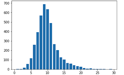
As you see the class distribution looks like the Gauss distribution, which we need to seperate the class like that

def ManualMap(x):
    array = [1, 3, 4, 5, 6, 7, 8, 9, 10, 11, 13, 16, 29]
    for i in range(len(array)):
        if x <= array[0]:
            return 0
        if array[i] <= x <= array[i + 1]:
            return i + 1
        if x >= array[-1]:
            return len(array)
        
def LogMap(x):
    array = np.around(np.geomspace(1, 29, 13))
    for i in range(len(array)):
        if x <= array[0]:
            return 0
        if array[i] <= x <= array[i + 1]:
            return i + 1
        if x >= array[-1]:
            return len(array)

d1 = pd.DataFrame(data["Rings"].map(ManualMap)) #[i for i in map(fun, data["Rings"])
# print(d1.shape, d1.columns)

counts = []
for i in range(1, 30):
    count = d1.loc[lambda df: df["Rings"] == i].shape[0]
    if count != 0:
        counts.append(count)

plt.subplot("121")
plt.bar(range(len(counts)), counts)
plt.xticks(range(len(counts)))
plt.xlabel("Seperate By ManualMap")

data["Rings"] = data["Rings"].map(LogMap) #[i for i in map(fun, data["Rings"])

counts = []
for i in range(1, 30):
    count = data.loc[lambda df: df["Rings"] == i].shape[0]
    if count != 0:
        counts.append(count)

plt.subplot("122")
plt.bar(range(len(counts)), counts)
plt.xticks(range(len(counts)))
plt.xlabel("Seperate By LogMap")

plt.tight_layout()
plt.show()

#data["Rings"] = d1

data = data.values.astype(np.float)

png

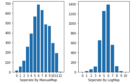
Here you can see that with ManualMap seperating the classes into 13 classes, and the result will be disperse.
While divide the class into 13 classes with LogMap, it looks more likely the Gauss distribution.

Model builting

from sklearn.svm import SVC
from sklearn.preprocessing import MinMaxScaler
from sklearn.model_selection import train_test_split, cross_val_score
from sklearn.ensemble import GradientBoostingClassifier


mms = MinMaxScaler()
mms.fit_transform(data[:, :-1])

X_train, X_test, y_train, y_test = train_test_split(data[:, :-1], data[:, -1], test_size=0.3)

def getScore(clf, X_test, y_test):
    yPre = np.round(clf.predict(X_test))
    # print(np.hstack((yPre, y_test.reshape(X_test.shape[0], 1))))
    acc = (yPre == y_test)
    print(f"{np.mean(acc) * 100:*^20}")


clf = SVC(gamma=10)
#clf = GradientBoostingClassifier(n_estimators=50, max_depth=2, learning_rate=0.5)

clf.fit(X_train, y_train)
getScore(clf, X_test, y_test)
getScore(clf, X_train, y_train)

print(cross_val_score(clf, X_test, y_test))

*54.066985645933016*
*54.567225453301404*
[0.5452381  0.51913876 0.56971154]

It turns out that seperate into 13 classes is still to many for the classifiers to work with.You can try the 3-classes method to retrain the model, and the accuracy will be better than 80%.
According to the offical suggestion, KNN and SVM working on the raw data, which has 20+ classes, get poor result.
BTW: If you want to get better result try manualy seperate with array[1, 3 ,5, 8, 11, 29]

Summary

The data sets beat me at the first place.For a long time, i have been working on Iris data set, which many classifier can do quite a good job.
It reminded me of the importance of the accuracy of the training set and cross_validation result

Data Analytics(2)